Generative models are a class of statistical models that try to learn the underlying structure of given data. This is different from discriminative models that try to discriminate between different types of data.

In machine learning, we assume the data X in any dataset comes from some underlying distribution p(X). When we are dealing with a supervised learning problem a data point x is associated with its corresponding label y, and data corresponding to each class of labels come from a different distribution P(X|Y).

For example, let’s say we want to train an image classifier that can classify a given image as ‘cat’ or ‘dog’. We will train this model using a dataset of images with each image x having a corresponding label y - either ‘cat’ or ‘dog’. This classifier is an example of a discriminative model since it tries to discriminate the images of cats and dogs.

On the other hand, if we want to generate new images of dogs, we will need a generative model that can learn the properties of the underlying distribution of dog images and then sample new images from that distribution.

In the paper An Introduction to Variational Autoencoders, the two types of models are described as follows:

While in discriminative modeling one aims to learn a predictor given the observations, in generative modeling one aims to solve the more general problem of learning a joint distribution over all the variables. A generative model simulates how the data is generated in the real world. “Modeling” is understood in almost every science as unveiling this generating process by hypothesizing theories and testing these theories through observations.

In math terms:

Generative models try to model the joint distribution p(X, Y) while discriminative models try to model p(Y|X). You can see how generative models can be very powerful and we can get discriminative models from them whenever we want by conditioning on the input data. Unfortunately, making a good generative model is very difficult, as it has a much harder job to do, and if all we want to do is predict the labels for the input data, then training a discriminative model is usually a much simpler process and requires less training data and time. It also makes intuitive sense that generative modeling is much harder than discriminative modeling - most people need to think a lot to decide which restaurant they want to go to for dinner, but if someone else makes suggestions it is easy to decide whether that would be a good choice or not.

Popular examples of generative models include Generative Adversarial Models (GANs), which we will see in the next sections, and Variational Autoencoders (VAEs).

Intro

GANs are generative models that try to learn the underlying distribution of a given dataset by making two sub-models compete against each other in a zero-sum game. For example, we might give the model a large number of images of human faces and then the GAN should hopefully learn to generate new realistic images of people that aren’t in the dataset. The two sub-models are called the generator and the discriminator.

The generator is the thing that does the generative modeling and tries to create new points that plausibly come from the same dataset. The discriminator tries to discriminate whether a particular image came from the real dataset or the generator.

Loss function

Since there are two different models in GANs that work against each other, we need two loss functions to train them, one for each.

For the discriminator, we want it to correctly classify the images being real (coming from the training dataset) or fake (generated by the generator), so we want to penalize incorrect predictions. We can use a simple binary cross entropy or BCE loss for this. In a batch of size N, if the correct label for the i^th image is \( y_i \) and the value predicted by the discriminator is \( \hat{y_i} \), then the loss becomes:

For the generator, we want the opposite, because we want the discriminator to incorrectly predict our generated images as real. We give the discriminator a set of generated images and penalize the generator for images that the discriminator correctly predicts as being fake. So in this case, the true labels (\( y_i \)) are 0 for all the examples and we want the predictions to be as close to 1 as possible, thus the loss function for the generator becomes:

Note: While implementing the generator loss yourself make sure you don’t update the weights of the discriminator during this step.

Training GANs

The training of a GAN involves two steps, which are alternated during the training process.

1. The discriminator trains on images generated by the generator mixed with real images from the dataset
2. The generator is trained based on the predictions given by the discriminator on the generated images.

In the beginning, neither the generator nor the discriminator knows what they are doing. The generator generates really bad images that look nothing like the dataset because it has no information about what the images should look like. As the discriminator slowly learns how to differentiate between real and fake images, it propagates that information to the generator in the form of generator loss that is based on how realistic each image looks to the discriminator. As the training process goes on, both the generator and the discriminator get better until eventually, the generator starts generating images that look real even to humans.

While the basic idea behind GANs is simple and intuitive, in practice many potential factors can lead to poor performance or unexpected results. Some of these issues are listed below -

Vanishing gradients

During training, the job of the discriminator is much easier compared to the generator. While the discriminator only has to correctly predict which image is real and which one is fake, the generator has to create a realistic image using just the noise vector as input. Because of this reason, the discriminator might learn much faster than the generator and start to correctly predict all the generated images as fakes. With traditional activation functions like sigmoid or tanh, the gradients become very small when the discriminator predicts ‘real’ or ‘fake’ with very high confidence. When that happens, the generator will not get any meaningful feedback to update its weights and improve, further exacerbating the problem making the generator stuck in a non-optimal place.

Some solutions proposed to deal with this issue include using Wasserstein loss or a modified minimax loss proposed in the original GAN paper.

Failure to converge

If you are familiar with reinforcement learning you might have seen another issue that might arise in this process. Both the generator and the discriminator are chasing non-stationary targets, which means that they might fail to converge. For example, take a simple image classification problem, there, the dataset is static, i.e., it does not change during the training process, and so the optimal weights that we are trying to reach are constant and we can use gradient descent to slowly reach that point. In a GAN, however, once the generator is updated, the images it will produce in the next step for the discriminator will be different, and so the target towards which the discriminator is trying to move is itself moving. Similarly, for the generator, as the discriminator gets better, the loss for the same generated image will keep changing.

Because of this, GANs frequently fail to converge. As mentioned in this google developers post, some regularization methods like adding noise to discriminator inputs and penalizing discriminator weights can be used to improve GAN convergence.

Mode collapse

Often the distribution of data that we are trying to capture with our GAN is multimodal, i.e., with more than one mode or peak in the distribution. For example, in the MNIST dataset, there are 10 classes (digits 0 to 9) and each of those corresponds to a mode in the distribution of that dataset, with the spread around those modes denoting the variation that can be found within each class.

During training, the discriminator might find it easier to distinguish between real and fakes of one class compared to others. Consequently, the generator might stop generating images of that class because it is easier to fool the discriminator in other classes. After a few steps like this, you might find that the generator is only generating images from one of the classes (the digit ‘1’ for example). This is called mode collapse.

You can deal with this issue using Wasserstein Loss or Unrolled GANs.

Measuring performance: FID

The basic idea behind Frechet Inception Distance or FID is that in order for the fake images to be indistinguishable from the real ones, they should come from the same distribution of images that we would consider real.

Let’s say we have a bunch of images that we generated using our GAN, or any other method of generating images, and we want to compare them to a set of real images to get a sense of how well our model did. One way to do this could be to manually look at some example images to get a general idea of what our model is producing.

While this is easy to do and gives us a feel of how good our model is, one might also want a more objective way to measure GAN performance to compare different models and to report their findings to others.

One such metric is the Frechet Inception Distance. FID is the distance between the distributions of real and fake images. The distance in this context is a measure of dissimilarity between the two distributions. To calculate the distance, we take the Inception V3 model, but instead of using the final classifications from the model (like in Inception Score), we use it as a feature extractor and take the activations from the last pooling layer of the model before the fully connected layers and see how the images are distributed in that space.

Calculating the distance

Here, we make the assumption that the distributions take the form of multivariate normal distributions which simplifies our calculation and makes computation easy.

A multivariate normal distribution can be parameterized by its mean vector \((\mu)\) and covariance matrix \((\Sigma)\).

The formula for calculating the distance is:

Here, tr(X) is the trace of the matrix X, and ||X|| is the norm of X. Distributions 1 and 2 are of the real and generated images respectively. Also, note that \( \sqrt{\Sigma_1\Sigma_2} \) is the square root of the resulting matrix \( \Sigma_1\Sigma_2 \) and not element-wise square root.

This has the dimensions of distance squared and gives us a measure of how far apart the two distributions are. The closer the two distances, the lower the FED and the better your generated images. We should use a large number of real and generated images for this calculation to reduce noise and get meaningful results from the calculation.

You can check out this blog post by Jason Brownlee for the Python implementation of the FID.

Advantages

1. This metric is easy to calculate once the images are generated.
2. It is based on the Inception model trained on the ImageNet dataset that covers a large variety of classes, so it is applicable in lots of use cases.
3. Unlike the Inception Score, it compares the distributions of the real and fake images, while the Inception Score only looks at the generated images.

Limitations

1. Requires a large amount of data (both real and fake images) to give good results.
2. Only good on tasks that are a subset of ImageNet, or close enough that the embeddings make sense.
3. Does not capture everything about the distributions, just the first two moments.
4. The metric is biased and depends on the number of samples, which limits its usefulness as a good metric to benchmark different GANs.

Measuring performance: Inception Score

The basic idea behind the Inception Score is that if a state-of-the-art image classifier thinks the images generated by your model are real, then they must be good.

To calculate the Inception Score, we use the Inception-V3 model to classify the generated images from our GAN, if the images are being classified into one of the classes with high confidence, then that is an indicator that the generated images are real looking. On the other hand, if the classifier is confused and can’t classify the generated images confidently, then perhaps the generated images are bad/low fidelity,

A good GAN will generate a large variety of real-looking images. Thus, the metric we use to assess the quality of the images should look at both of these factors - high fidelity and diversity.

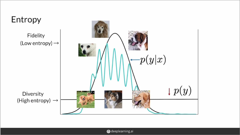
High fidelity

Looking at fidelity, for a given image x, the model predicts the distribution p(y|x) over the possible classes y. We want this distribution to have a high value for a few classes (or ideally just one class) and very low for others, which would suggest that the model is very confident in classifying the image, while for a bad/low fidelity image we might expect the classifier to not be very sure about what is in the image and thus give a distribution closer to a uniform distribution. Another way of saying the same thing would be that we want the entropy of p(y|x) to be as low as possible.

Here entropy means the uncertainty or randomness in the outcome of the random variable. A well-made fake image of a dog is very likely to be predicted as a dog, so there will be less uncertainty in the outcome, and thus, low entropy.

Diversity

It is also important that the model produces a diverse set of images, and we want the generated images to be more or less uniformly distributed across all classes, another way of thinking about it is that without seeing the generated image, we should have no idea what the classifier would predict, and thus the entropy of p(y) should be high. Notice that this time we didn’t condition it on a given x.

So, to summarize, we want the entropy of the distribution p(y|x) to be low and that of p(y) to be high. These two things signify different aspects of what makes a GAN good. Think about how in a classifier, the precision and recall signify different aspects of the classifier that we combine to create the F1 score. Similarly, when we combine the two values we described above, we get the Inception Score.

Calculating the Inception Score

To capture the fidelity and diversity in a single number, we want to calculate the dissimilarity or distance between the two distributions, in the form of KL divergence, also called relative entropy.

Note that while we can think of KL divergence as distance, strictly speaking, it is not a measure of distance because it is not symmetric, i.e., \( D_{KL}(P||Q) \neq D_{KL}(Q||P) \) in general. Decreasing the entropy of p(y|x) or increasing the entropy of p(y) would both result in the KL divergence going up.

Now, we can average over the generated images x by taking the expectation. Finally, we take the exponent of this number to make the result easier to compare. So the complete formula then becomes:

You can check out this blog post by Jason Brownlee for the Python implementation of the IS.

Limitations

While the Inception Score takes into consideration the diversity of classes in the images produced, it does not look at diversity within a particular class, so this method will still give us a good score if our model creates just one very realistic image in each class.

Also, similar to FID, it uses the Inception model which is trained on the ImageNet dataset, so if we are trying to generate images that are different from the kind of images found in that dataset, scores given by the classifier might not be very useful. It is entirely possible that a real-looking image doesn’t get a good prediction from the inception classifier, or conversely, a good score is given for a fake-looking image.

Another important issue is that the Inception Score doesn’t look at any real images to compare against, so it provides no information about how close our generated images are to the kind of images that we want to generate.

References

1. [1906.02691] An Introduction to Variational Autoencoders (arxiv.org)

2. Background: What is a Generative Model? (google.com)

3. Generative Models (openai.com)

4. Build Basic Generative Adversarial Networks (GANs) | Coursera

5. Build Better Generative Adversarial Networks (GANs) | Coursera

6. GAN Training | Generative Adversarial Networks | Google Developers

7. Common Problems | Generative Adversarial Networks | Google Developers

8. [1406.2661] Generative Adversarial Networks (arxiv.org)

9. GANs Trained by a Two Time-Scale Update Rule Converge to a Local Nash Equilibrium (arxiv.org)

10. [1606.03498] Improved Techniques for Training GANs (arxiv.org)

11. How to Implement the Frechet Inception Distance (FID) for Evaluating GANs (machinelearningmastery.com)

12. Fréchet inception distance - Wikipedia

13. How to Implement the Inception Score (IS) for Evaluating GANs (machinelearningmastery.com)

14. Kullback–Leibler divergence - Wikipedia