
Normalization Methods
Published:
Normalization is the process of transforming the features of a dataset so that they are all on the same scale. Features having very different scales can make the process of training harder by creating regions of flat gradients where the training can get stuck. Normalization involves taking a feature, subtracting the mean value, and then dividing it by the standard deviation so that the new transformed value has zero mean and unit variance.
Deep neural networks have a large number of layers and are typically trained for many epochs. Even if the input data is normalized before training, as each layer applies non-linear transformations to its inputs, the outputs of the deeper layers – which serve as the inputs for the next layers – can start diverging from the normal distributions over the epochs. This phenomenon is known as internal covariate shift which can cause the training to slow down and reduce the performance of the model.
Normalization methods
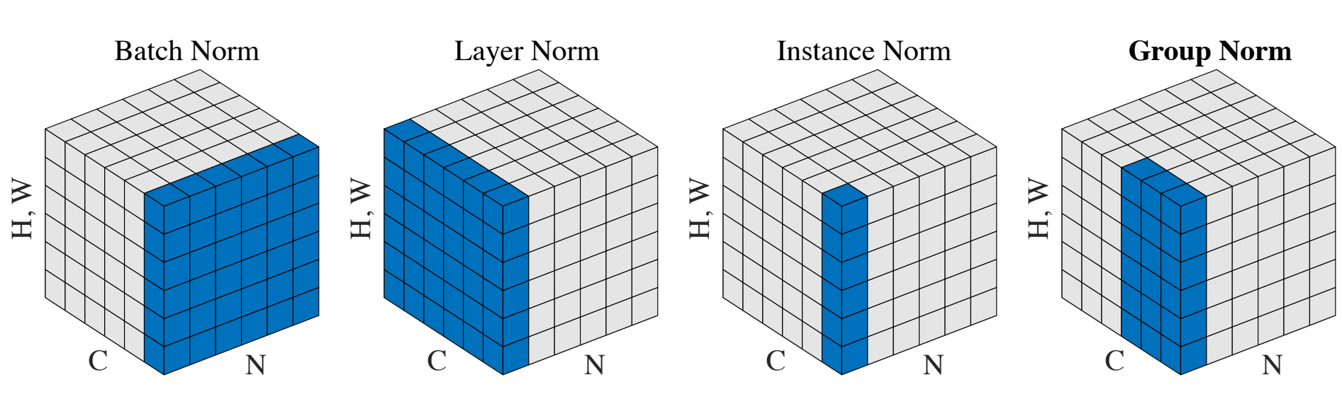
For normalizing the outputs of intermediate layers, there are several methods that can be used based on the model and use case. Some common normalization methods are:
- Batch Normalization
- Layer Normalization
- Instance Normalization
- Group Normalization
Batch Normalization
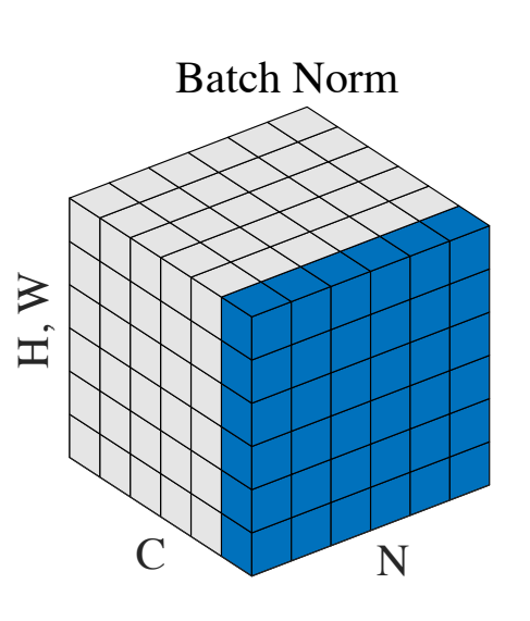
This is one of the most common normalization methods. Batch norm normalizes the features along the batch dimension, i.e., it calculates the mean and standard deviation for each feature using a mini-batch. If we keep the batch size sufficiently large (e.g., 32 or more), then the batch statistics are a reasonable substitute for the statistics of the entire dataset.
Let’s take the example of training for a vision task given in the paper for Instance Normalization where the images come in batches of shape \(T \times C \times W \times H\). Here,
- T is the number of images in a batch
- C is the number of channels (e.g., 3 channels of color images)
- WxH are the spatial dimensions of the image.
For input value \(x_{tijk}\) batch normalization converts it into the output \( \hat{x}_{tijk} \) in the following way:
\[\hat{x}_{tijk} = \frac{x_{tijk} - \mu_i}{\sqrt{\sigma^2_{i} + \epsilon}}\]Where,
\[\mu_i = \frac{1}{HWT}\sum^{T}_{t=1}\sum^{W}_{l=1}\sum^{H}_{m=1}x_{tilm}\] \[\sigma^2_i = \frac{1}{HWT}\sum^{T}_{t=1}\sum^{W}_{l=1}\sum^{H}_{m=1}(x_{tilm} - \mu_i)^2\]The statistics are stored along with the model and at inference time the pre-computed values for mean and variance are used to transform input data.
This introduces dependence between the different data points during training. Another issue is that if the batch size becomes small due to memory limitation, then the performance of the model can degrade significantly.
Layer Normalization
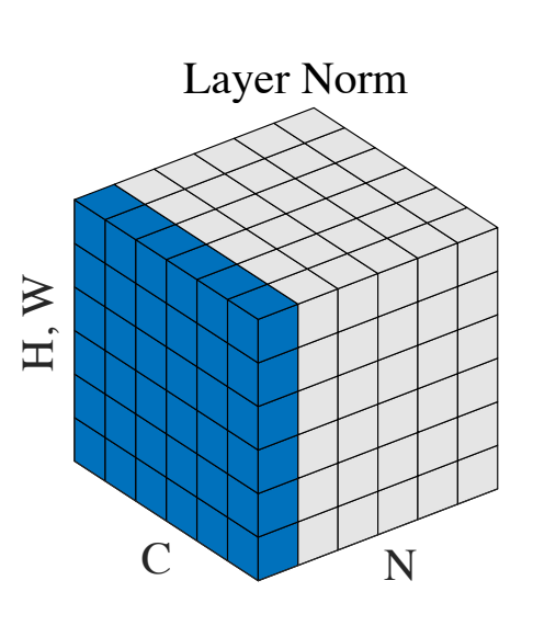
To avoid the limitations of batch norm, the layer norm technique can be used. Instead of normalizing across a batch of data points, layer norm acts on individual data points by normalizing across the feature dimension.
This avoids several limitations of batch norm since it is not dependent on batch size and does not introduce dependencies between different data points in a batch. The idea is that internal covariate shift can be mitigated by normalizing within a layer since the inputs to the next layer are highly correlated to the outputs of the first layer.
Using the same notation as above, layer norm can be written as follows:
\[\hat{x}_{tijk} = \frac{x_{tijk} - \mu_{t}}{\sqrt{\sigma^2_{t} + \epsilon}}\]Where,
\[\mu_{t} = \frac{1}{HWC}\sum^{C}_{i=1}\sum^{W}_{l=1}\sum^{H}_{m=1}x_{tilm}\] \[\sigma^2_{t} = \frac{1}{HWC}\sum^{C}_{i=1}\sum^{W}_{l=1}\sum^{H}_{m=1}(x_{tilm} - \mu_{t})^2\]Instance Normalization
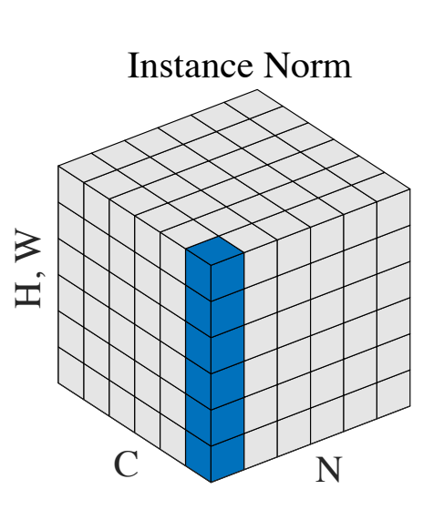
With instance normalization, each feature is normalized separately. The idea behind instance norm is that values in different channels/features could have very different statistics and normalizing all values using the combined statistics of all the features might not be the best idea.
For instance, in an image, there are many channels at any given intermediate layer, which are created using their own separate kernels. So only individual channels should be normalized. This way, contrast can be normalized in the images.
Instance norm can be written in the following way:
\[\hat{x}_{tijk} = \frac{x_{tijk} - \mu_{ti}}{\sqrt{\sigma^2_{ti} + \epsilon}}\]Where,
\[\mu_{ti} = \frac{1}{HW}\sum^{W}_{l=1}\sum^{H}_{m=1}x_{tilm}\] \[\sigma^2_{ti} = \frac{1}{HW}\sum^{W}_{l=1}\sum^{H}_{m=1}(x_{tilm} - \mu_{ti})^2\]Group Normalization
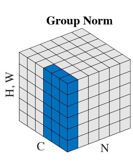
Group normalization can be thought of as being a middle ground between layer norm and instance norm. Group norm divides the channels into different groups and then normalizes across the channels in different groups separately.
Consider the sub-image containing channels from only one group, if we apply layer norm on that sub-image, and then repeat the process for every group, we get group norm.
Group norm can be written in the following way:
\[\hat{x}_{tijk} = \frac{x_{tijk} - \mu_{tu}}{\sqrt{\sigma^2_{tu} + \epsilon}}\]Where,
\[\mu_{tu} = \frac{1}{HWG_u}\sum^{W}_{l=1}\sum^{H}_{m=1}\sum_{i \in \mathbb{G_u}}x_{tilm}\] \[\sigma^2_{tu} = \frac{1}{HWG_u}\sum^{W}_{l=1}\sum^{H}_{m=1}\sum_{i \in \mathbb{G_u}}(x_{tilm} - \mu_{tu})^2\]Here, \( G_u \) is the size of group \(u\) and \( \mathbb{G_u} \) is the set with all the channels in group \(u\).
Layer norm and instance norm can be seen as special cases of group norm. If the number of groups is 1, then group normalization is equivalent to layer norm, and if the number of groups is the same as the number of channels, i.e., each group has only one channel, then it is equivalent to instance norm.
Further Processing
Once \( x \) is normalized to create \(\hat{x}\), we can rescale the values for different channels in the following way:
\[y_i = \gamma_i \hat{x}_i + \beta_i\]Where \(\gamma_i\) and \(\beta_i\) are learned parameters. This compensates for possible loss of representational ability that might have occurred due to normalization, making sure performance does not degrade.
Leave a Comment