The transformer is a deep learning model used primarily for Natural Language Processing tasks, such as machine translation, but is slowly also finding use in tasks like computer vision with models like Vision Transformer. Several of the biggest and best-performing language models like BERT and GPT-2/GPT-3 are transformer based models. The architecture was introduced in the paper Attention Is All You Need. In this post we will follow the paper closely along with this post from Jay Alammar.

On a high level, transformers are encoder-decoder models, so the input strings (which can be of variable lengths) go through the encoder and get converted to a fixed-length representation in a latent space. This latent representation then goes through the decoder and gives us the desired output, which might also be of variable length.

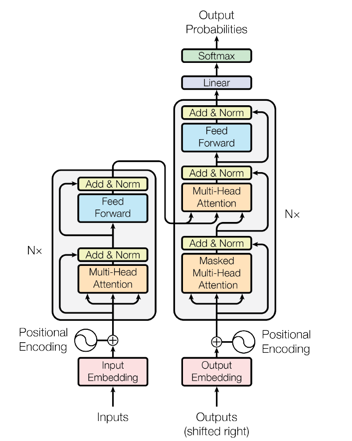
Let’s say we want to translate the sentence “The transformer is a powerful and versatile machine learning model.” into German, which translates to “Der Transformator ist ein leistungsstarkes und vielseitiges Modell für maschinelles Lernen.” (I don’t know German, I used Google Translate for this). For our model to translate the source sentence into the target sentence, it will first need to encode it into some latent representation, this encoding step essentially extracts out the meaning of the sentence, which can then be used to convert it into a sentence in another language. In the second stage, the decoder takes this latent representation and generates the translated sentence one word at a time. The full architecture is shown below, we will see each of these components in detail in the coming sections.

Inputting data

The raw data we have is in the form of sentences, which are ordered lists of words. We convert them to an ordered list of tokens using the vocabulary we have for the language. These lists of numbers can be padded to some maximum length, and then batched to create BxN matrices, where B is the batch size and N is the maximum length of sentences. These tokens are then converted to embeddings of dimensions D, converting the sentence into a matrix of shape NxD, and thus making the batch a rank-3 tensor of shape BxNxD. Working with tensors like this makes computation much more efficient, especially on GPUs which are made to do a lot of large matrix operations as efficiently as possible.

Positional Encoding

Now that we have represented our sentences as matrices, we also need to encode the positional information of each word and combine it with the embeddings created in the previous step. Traditionally with LSTMs, the positional information of a word is implicitly present in the encoding as a result of sequentially processing the input sentence, but if we can store that information in the word embedding itself, it will allow us to process all the words of a sentence in parallel and still have information about each word’s position in the sentence.

For every position in the sentence, we need to create a representation that encodes the information about that position. Here, we have the option of using pre-defined encodings or learning them during training. If we create a P dimensional vector for encoding a given position in the sentence, then for a sentence of maximum length N, the positional encoding will be a matrix of size NxP.

But how do we combine this information with the word embeddings to have a unified representation that has information about both the word as well as its position? One way is to concatenate the positional embedding with the word embedding, making the final representation of each word a (D+P) dimensional vector, and thus the representation of a complete sentence will be a matrix of shape Nx(D+P). We can see this increases the complexity of our model and thus increase the memory and compute requirement for training.

Another way is to simply add the positional encodings to the word embeddings. This might not seem like a good idea at first but the authors of the paper found this method to work very well and it also decreases the complexity of the model. For more detailed discussion check out this video by AI Coffee Break with Letitia. Recently, alternative ways like introducing linear biases in the attention scores have been proposed that can improve performance on test sequences longer than those encountered during training (see ALiBi).

For now, we will just add the positional encoding to the word embeddings, which means their dimensionality needs to be the same, i.e., P=D. This also saves us the trouble of having to tune another hyperparameter during training. In terms of whether we should use pre-made or learned positional encodings, the authors tried both and found that there was no significant difference in performance between the two methods, and finally decided to use the pre-defined encodings because those would likely generalize better to sentences longer than the ones found in the training data.

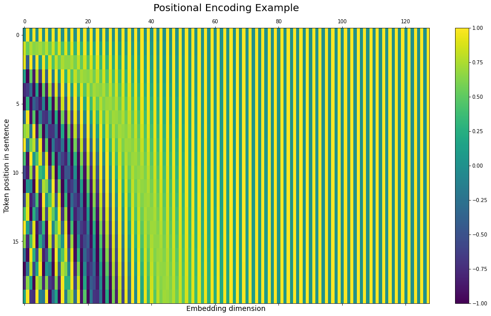
The formula used for positional encoding is as follows:

Here, pos is the position of the word, and 2i represents the even dimensions while 2i+1 represents the odd dimensions in the encoding. The positional encodings are generated by interleaving sine and cosine functions of different frequencies for different dimensions. This representation does not look very intuitive at first glance, but it looks somewhat like a Fourier Transform, so we can think of it as bringing the information of time domain - i.e., position in the sentence, into the space domain - i.e., word embedding.

The authors of the paper explain the choice of this function as follows:

We chose this function because we hypothesized it would allow the model to easily learn to attend by relative positions, since for any fixed offset k, PE_pos+k can be represented as a linear function of PE_pos.

So now, we have word embeddings and positional encodings, and after adding these two we arrive at the final representation of our batch of sentences with the shape BxNxD that are ready to be input into the encoder and start the translation process.

Attention

Unlike classical RNN models like LSTMs, attention works in a way that can be easily parallelized and processed efficiently on GPUs, significantly improving scalability for larger language models.

Attention is at the core of the transformer model and it’s what makes the model perform as well as it does. This is evident in the fact that the paper introducing the transformer architecture is titled “Attention is all you need”.

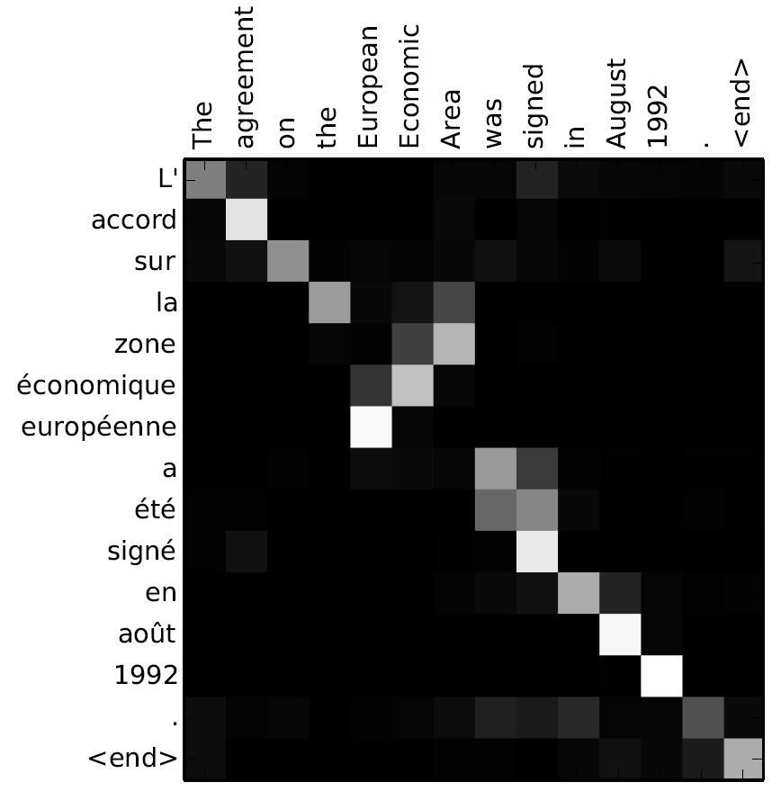
To understand what attention is, let’s go back to our example - we want to encode our sentence “The transformer is a powerful and versatile machine learning model”. While encoding each word, we need to look at other words in the sentence to gather the complete meaning of that word. When encoding the word “powerful”, we also want to know what is the thing we are calling powerful - “The transformer”. Attention is the mechanism that the transformer model uses to gain this ability of understanding relationships between different words of a sentence.

The way attention works is that for each word, we create 3 vectors: Query, Key, and Value vectors. These vectors are created by using three trainable matrices W^Q, W^K, and W^V of shapes DxD_K, DxD_K, and DxD_V respectively. For a sentence of N words, this translates to doing a matrix multiplication between the NxD matrix containing our sentence and these three matrices, giving us the Q, K, and V matrices of respective dimensionality NxD_K, NxD_K, and NxD_V.

Where,

By multiplying the Query matrix and the transpose of the Key matrix, we get the NxN attention matrix which tells the model how much “attention” to pay to each word while encoding a particular word. We can see that this matrix multiplication means the shapes of the matrices Q and K must be the same.

Dot-Product Attention

Let’s look at these matrices in a little bit more detail. In the attention matrix, the value of the (i, j)^th cell is the dot product of the i^th row in the Q matrix and j^th row in the K matrix. The Query matrix Q stores the “queries” - what information is the word looking for in the other words in the sentence? The Key matrix K stores the “keys” - what information can that particular word provide? Since the dot product gives us a measure of similarity between two vectors, we can think of the value of the (i, j)^th cell as the relevance of word j while encoding word i in the sentence i.e. a measure of how much information relevant to the word being encoded is provided by the word being queried.

Finally, softmax is applied to this matrix to normalize the attention values such that the “relevance scores” of all the words used for encoding a particular word add up to 1. In practice, the matrix is also divided by the square root of the size of key vectors (\( \sqrt{D_K} \)) before the softmax step , this scaling helps to prevent the values from going into regions of the softmax function with extremely small gradients. This attention matrix is finally multiplied by the Value matrix so that now each word’s encoding is a sum of encodings of the input words scaled by their relevance. The final formula for dot-product attention thus becomes:

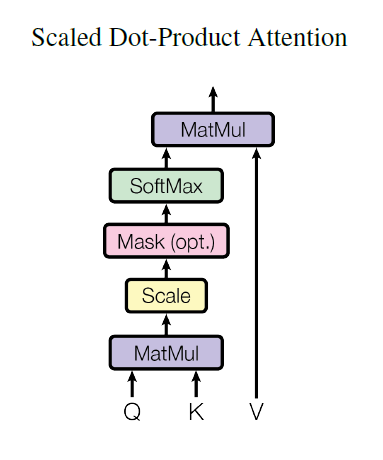
While implementing this in batch settings, with the input of shape BxNxD, we can use functions like torch.bmm in PyTorch, which does the matrix multiplications independently for the B sentences in our batch and gives us the final output of the shape BxNxD_V

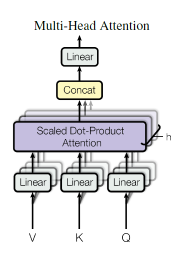
Multi-head attention

We saw how attention calculates the “relevance scores” of different words and thus how much attention to pay to them while encoding our sentence, but there can be lots of different aspects of what relevant means. It could relate to the grammatical structure of the sentence, or the gender of different words, or many other things. To capture these different aspects of the relationship between different words, we can perform the steps of calculating attention multiple times in parallel, with different W^Q, W^K, and W^V matrices that are all randomly initialized at the start of the training process. Then during training, these different “heads” of attention can hopefully learn these different aspects of attention.

Think of these different attention heads like different channels in a convolution layer of ConvNets, with each channel having its own kernel that encodes a different aspect of an image.

So now, if we have h attention heads, we get h outputs of attention with shape NxD_V. To combine them, we simply concatenate them giving us an output of shape Nx(hD_V). Finally, we multiply this with a weights matrix (W^O) of shape (hD_V)xD which projects the attention values in the space of the word embeddings, giving us the final output of multi-head attention in the shape NxD, which is what the downstream layers are expecting.

Once again, while implementing this in a batch setting we will use batch matrix multiplication giving us the output of shape BxNxD.

Encoder

The encoder consists of several encoder blocks, which have the same architecture but do not share weights. Think of them as the hidden layers in a dense neural network, or like convolution + max-pooling blocks in a ConvNet. Each additional encoder block adds the ability for the model to learn higher-level representations of the text. The encoder block contains a self-attention sub-layer and a feed-forward neural network sub-layer. There are residual connections and layer normalization steps after both sub-layers. Let’s see each one of them in more detail.

Self-Attention

We have seen how attention works in the previous section. Self-attention is when the Query, Key, and Value matrices all come from the same sentence. So while encoding the input sentence, we are calculating the self-attention, or how much attention to pay to the words of the input sentence while encoding a particular word. This is slightly different from the implementation of attention in the decoder layer which we will see later.

Feed-Forward Neural Network

After getting the output from the attention layer, it goes through a fully connected feed-forward neural network. Each word goes through this network separately and identically. There are two layers in this network with a ReLU activation after the first layer. The first layer has an output of shape D_ff which is another tunable hyperparameter of this model. The second layer has an output of shape D, so that the final output of this sub-layer has the same shape as the input.

Residual + LayerNorm

A residual connection means to simply add the input to the output of a given function.

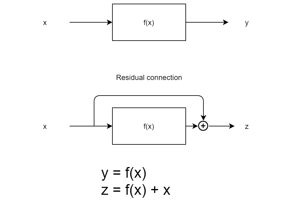
After getting the output of the sublayers, we apply a residual connection and then apply layer normalization to the output of the residual.

Final result

Putting all of these together, the output of the encoder block looks something like this:

Where,

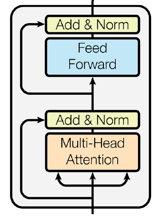
The complete encoder is a stack of multiple encoder blocks like this, with each encoder block giving an output of the same shape as its input, but internally the sentence is transforming from containing the embeddings of individual words to containing a high-level abstract meaning of the whole sentence.

Decoder

The decoder works very similarly to the encoder, with a few important differences. Like the encoder, the decoder is also a stack of multiple decoder blocks with the same architecture but different weights. However, in a decoder block, there are two attention sub-layers before the feed-forward sub-layer.

Masked Self-Attention

The first attention sublayer is also a multi-head self-attention sublayer, but this time, a word is only allowed to attend to itself and the words before it, and no words that come after it. This is done by masking the future words, i.e., by replacing the values of the cells (i, j) where (j > i) in the attention matrix (\( Q \times K^{T} \)) with -infinity before the softmax step. This means that after the softmax step, the attention value of future words will become zero.

This is done because while creating the translated sentence, we start with an empty sentence and create the sentence one word at a time until a special end-of-sentence character is generated or the maximum length of the output sentence is reached.

Encoder-Decoder Attention

The second attention sub-layer is not self-attention, rather, it creates the Query matrix using the output from the previous masked self-attention layer and Key and Value matrices using the output from the encoder, i.e., output from the last encoder block in the encoder stack. If the maximum sentence length of the output sentence is M, then a sentence is represented as an MxD matrix, which is also the shape of the output from the masked self-attention sub-layer. Using this, we get the Query matrix of shape MxD_K, while the K and V matrices come from the encoder and have shapes NxD_K and NxD_V respectively. This gives us the attention matrix of shape MxN. Finally, this process gives us the Value matrix of shape MxD_V. Concatenating the results of multiple attention heads and multiplying with the weights matrix like in the case of the encoder gives us the final output of shape MxD. M and N can be different if required but M=N usually also works well. The embedding dimension (D) must be the same for both the source and target language.

Feed-Forward NN and Residual + LayerNorm

Once again, like the encoder, we have a feed-forward neural network with an intermediate layer with shape D_ff and ReLU activation and a final layer of shape D. Similar to the encoder, all these sub-layers have residual and layer norm components, so the complete output of a decoder block becomes:

Where,

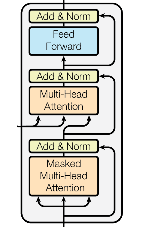
Once again, the decoder consists of multiple decoder blocks stacked on top of one another.

Final Result

After multiple decoder blocks as described above, we finally get to the linear + softmax layer to generate the output tokens. The linear layer takes us from the D dimensional embedding space to a V dimensional space, where V is the vocabulary size of the target language. Each dimension in this space corresponds to one word in the target language. We apply softmax to this result which converts the output into probabilities of different words. Now, we can get the generated token either by taking the word with the highest probability or by sampling randomly using the probability values given by the softmax layer.

Putting it together

Let’s look at the entire process in one place.

1. The input sentence is turned into embeddings.
2. Positional encodings are added to the sentence embeddings to create the input for the encoder.
3. Multiple encoder blocks are stacked where each block has the following components-
   1. Multi-head self-attention followed by residual + layernorm
   2. Fully connected feed-forward network followed by residual + layernorm
4. Embeddings are created for the target sentence decoded so far (starts with an empty sentence []).
5. Positional encodings are added to the embeddings of the target sentence.
6. Multiple decoder blocks are stacked where each block has the following components-
   1. Masked multi-head self-attention followed by residual + layernorm.
   2. Multi-head encoder-decoder attention followed by residual + layernorm.
   3. Fully connected feed-forward network followed by residual + layernorm.
7. Linear + softmax layer that finally gives the probabilities of the output words.

Hyperparameters

All in all, we have the following hyperparameters and the values for each used by the authors of the paper:

1. D - Embedding dimension = 512
2. h - Number of attention heads = 8
3. n_enc - Number of encoder blocks = 6
4. n_dec - Number of decoder blocks = 6
5. D_ff - Dimension of feed-forward layer = 2048
6. Dropout - Dropout rate for embeddings and output of each sub-layer = 0.1

Training

Optimizer

The authors of the paper used Adam optimizer.

Regularization

Dropout is applied to the output of each sub-layer before the residual + layernorm step. Dropout is also applied to the sum of embeddings and positional encodings for both encoder and decoder stacks.

References

1. [1706.03762] Attention Is All You Need (arxiv.org)
2. The Illustrated Transformer – Jay Alammar – Visualizing machine learning one concept at a time. (jalammar.github.io)
3. [1409.0473] Neural Machine Translation by Jointly Learning to Align and Translate (arxiv.org)
4. LSTM is dead. Long Live Transformers! - YouTube
5. The Annotated Transformer (harvard.edu)
6. Adding vs. concatenating positional embeddings & Learned positional encodings - YouTube